95 Fundamentals -- eigenvalue problem, Cayley-Hamilton theorem and the invariants of tensors

After previous episodes, I believe our readers have more understanding about what a tensor is. The concept of invariant is built in tensor itself -- a tensor is invariant to changes in coordination systems. However, the decomposition of a tensor $\textbf{T}$ is not invariant. $T_{ij}\neq T_{ij}'$ unless it is an isotropic tensor. Is it possible that there are something associated with a tensor that are also invariant to changes in coordination systems? That's what we are going to find out today!

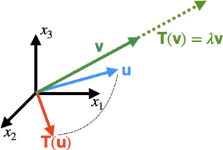
Eigenvalues and Eigenvectors

From previous episode, we know that a second-order Cartesian tensor can a linear mapping of vectors. Usually, these vectors will change their directions after the mapping. However, there are some vectors that are kind of "intrinsic" to the tensor. These "intrinsic" vectors will not change their directions after the mapping of the tensor. We call these vectors "eigenvectors," where "eigen" means "own." The relative length change after the mapping of the eigenvector is its associated "eigenvalue," which we denote as $\lambda$.

It is quite easy to solve eigenvalues and eigenvectors. From its definition:

$\textbf{T}\textbf{v}=\lambda\textbf{v},\quad(\textbf{T}-\lambda\textbf{I})\textbf{v}=0$

In order to have a nontrivial solution of $\textbf{v}$, the matrix $(\textbf{T}-\lambda\textbf{I})$ has to be singular (i.e., its determinant has to be 0, and thus cannot be inverted). Thus for a second-order Cartesian tensor with eigenvalues $\lambda_1, \lambda_2, ..., \lambda_n$, we can define the characteristic polynomial of tensor $\textbf{T}$ to be:

$p_{\textbf{T}}(\lambda)=\text{det}(\lambda\textbf{I}-\textbf{T})=(\lambda-\lambda_1)(\lambda-\lambda_2)...(\lambda-\lambda_n)$

The Characteristic Polynomial

For a second-order Cartesian tensor in a 3-dimensional space, we can expand every terms in the characteristic polynomial:

$p_{\textbf{T}}(\lambda)=\text{det}(\lambda\textbf{I}-\textbf{T})=\lambda^3-(T_{11}+T_{22}+T_{33})\lambda^2+(T_{11}T_{22}-T_{12}T_{21}+T_{11}T_{33}-T_{13}T_{31}+T_{22}T_{33}-T_{23}T_{32})\lambda-(T_{11}T_{22}T_{33}+T_{21}T_{32}T_{13}+T_{12}T_{23}T_{31}-T_{13}T_{31}T_{22}-T_{23}T_{32}T_{11}-T_{33}T_{12}T_{21})$

We can simplify it into:

$p_{\textbf{T}}(\lambda)=\lambda^3-\text{tr}(\textbf{T})\lambda^2+(\begin{vmatrix}T_{11}&T_{12}\\T_{21}&T_{22}\end{vmatrix}+\begin{vmatrix}T_{22}&T_{23}\\T_{23}&T_{33}\end{vmatrix}+\begin{vmatrix}T_{11}&T_{13}\\T_{31}&T_{33}\end{vmatrix})\lambda-\text{det}(\textbf{T})$

Since the solution of $p_{\textbf{T}}(\lambda)=0$ is $\lambda_1, \lambda_2, \lambda_3$, the characteristic polynomial can also be expressed as:

$p_{\textbf{T}}(\lambda)=\lambda^3-(\lambda_1+\lambda_2+\lambda_3)\lambda^2+(\lambda_1\lambda_2+\lambda_2\lambda_3+\lambda_1\lambda_3)\lambda-\lambda_1\lambda_2\lambda_3$

From direct comparison, we can thus define 3 indices for tensor $\textbf{T}$:

$I_{1}(\textbf{T})=\text{tr}(\textbf{T})=(\lambda_1+\lambda_2+\lambda_3)$

$I_{2}(\textbf{T})=\begin{vmatrix}T_{11}&T_{12}\\T_{21}&T_{22}\end{vmatrix}+\begin{vmatrix}T_{22}&T_{23}\\T_{23}&T_{33}\end{vmatrix}+\begin{vmatrix}T_{11}&T_{13}\\T_{31}&T_{33}\end{vmatrix}=\frac{1}{2}((\text{tr}(\textbf{T}))^2-\text{tr}(\textbf{T}^2))=\lambda_1\lambda_2+\lambda_2\lambda_3+\lambda_1\lambda_3$

$I_{3}(\textbf{T})=\text{det}(\textbf{T})=\lambda_1\lambda_2\lambda_3$

However, what will happen to these polynomial and indices if we change our coordinate system? From our tensor transformation rule, we know that:

$p_{\textbf{T}}(\lambda)=\det(\lambda\textbf{I}-\textbf{T})=\det(\lambda\delta_{ij}-T_{ij})=\det(\lambda LIL^T-LT'L^T)=\det(L)\det(\lambda I-T')\det(L^T)=\det(\lambda I-T')=\det(\lambda\delta_{ij}'-T_{ij}')$

Here we used the fact that $(\det(L))^2=1$. We show that the characteristic polynomial is invariant to coordination changes. Since the three indices we just defined previously are the coefficients in the characteristic polynomial, all three indices are invariant to coordination changes as well. These 3 special indices are called the "principal invariants of tensors."

We should pay some extra attention to our second principal invariant:

$I_2(\textbf{T})=\frac{1}{2}((\text{tr}\textbf{T})^2-\text{tr}(\textbf{T}^2))=\frac{1}{2}(T_{ii}^2-T_{ij}T_{ji})$

Since $T_{ii}$ is simply the first principal invariant, we can deduce that $T_{ij}T_{ji}$ is also an invariant. Similarly, $T_{ij}T_{ij}=\textbf{T}:\textbf{T}$ is also an invariant.

Cayley-Hamilton theorem

From previous definition of characteristic polynomial, we know that if we substitute $\lambda$ with any eigenvalue $\lambda_i$, the characteristic polynomial will vanish. Since the eigenvalues are kind of "intrinsic" to our original tensor, what will happen if we substitute $\lambda$ with our tensor $\textbf{T}$?

$p_{\textbf{T}}(\textbf{T})=\textbf{T}^3-I_1(\textbf{T})\textbf{T}^2+I_2(\textbf{T})\textbf{T}-\det(\textbf{T})\textbf{I}=?$

Since $p_{\textbf{T}}(\textbf{T})$ is a tensor, we will see how it will map our eigenvector $\textbf{v}_i$ with eigenvalue $\lambda_i$:

$p_{\textbf{T}}(\textbf{T})\textbf{v}_i=\textbf{T}^3\textbf{v}_i-I_1(\textbf{T})\textbf{T}^2\textbf{v}_i+I_2(\textbf{T})\textbf{T}\textbf{v}_i-\det(\textbf{T})\textbf{I}\textbf{v}_i$

$=\lambda_i^3\textbf{v}_i-I_1(\textbf{T})\lambda_i^2\textbf{v}_i+I_2(\textbf{T})\lambda_i\textbf{v}_i-\det(\textbf{T})\textbf{v}_i$

$=(\lambda_i^3-I_1(\textbf{T})\lambda_i^2+I_2(\textbf{T})\lambda_i-\det(\textbf{T}))\textbf{v}_i=\textbf{0}$

From theorem we are not going to prove here: if an nxn matrix has n distinct eigenvalues, the matrix has a basis for eigenvectors for $\Re^n$. That means for any vector $\textbf{u}$, we can express it in terms of the linear combination of the eigenvectors (i.e., $\textbf{u}=\alpha_i\textbf{v}_i$). Therefore, for any vector $\textbf{u}$,

$p_{\textbf{T}}(\textbf{T})\textbf{u}=\textbf{0}$

That means:

$p_{\textbf{T}}(\textbf{T})=\textbf{T}^3-I_1(\textbf{T})\textbf{T}^2+I_2(\textbf{T})\textbf{T}-\det(\textbf{T})\textbf{I}=\textbf{0}$

And this is the Caylay-Hamilton theorem. (This theorem also holds for degenerate tensors, but the proof requires a few more steps, which we will not go through here.)

From this theorem we can make the calculation of determinant and matrix inverse simpler. If we take the trace of $p_{\textbf{T}}(\textbf{T})$, we will get:

$\text{tr}(\textbf{T}^3)-\text{tr}(\textbf{T})\text{tr}(\textbf{T}^2)+\frac{1}{2}(\text{tr}(\textbf{T})^2-\text{tr}(\textbf{T}^2))\text{tr}(\textbf{T})-3\det(\textbf{T})=0$

$\det(\textbf{T})=\frac{1}{3}(\text{tr}(\textbf{T}^3)+\frac{1}{2}\text{tr}(\textbf{T})^3-\frac{3}{2}\text{tr}(\textbf{T})\text{tr}(\textbf{T}^2))$

By similar means, if we multiply $p_{\textbf{T}}(\textbf{T})$ to the tensor inverse of $\textbf{T}$, we will get:

$\textbf{T}^2-\text{tr}(\textbf{T})\textbf{T}+\frac{1}{2}(\text{tr}(\textbf{T})^2-\text{tr}(\textbf{T}^2))\textbf{I}-\det(\textbf{T})\textbf{T}^{-1}=0$

$\textbf{T}^{-1}=\frac{1}{\det(\textbf{T})}(\textbf{T}^2-\text{tr}(\textbf{T})\textbf{T}+\frac{1}{2}(\text{tr}(\textbf{T})^2-\text{tr}(\textbf{T}^2))\textbf{I})$

And we now have the inverse of a tensor!

Some Wrap Up

So in this episode, we first introduce the basic concepts of eigenvalue problems. We introduced the characteristic polynomial, and we showed that this polynomial is linked to the 3 principal invariants of a tensor. We also talked about Cayley-Hamilton theorem, and how this theorem can help us determine the determinant and the inverse of a tensor. That's a lot for a single episode, and I hope you enjoy so far. In our next episode, we will finally talk about something about stress and strain, so stay tuned!